Yes, it is a kernel.
A kernel is a way to measure similarity between two things. A function \(k(x, z)\) is a kernel if we can imagine mapping each input \(x\) to some possibly huge list of numbers called a feature vector and then \(k(x, z)\) just computes the dot product a standard way of measuring similarity between those two feature vectors. In this question we have a function and the size of the intersectionof the sets of words in the two documents\[ k(x, z) \;=\; \lvert \,\text{words}(x) \;\cap\; \text{words}(z) \rvert, \] which counts how many words document \(x\) and document \(z\) have in common. If both documents use the same set of words, then \(k(x, z)\) will be larger because it counts every word they share. Imagine there’s a dictionary of size \(D\). Each document \(x\) can be turned into a 0-1 vector of length \(D\). That means: 1.For the 1st dictionary word, set the 1st position to 1 if the document contains that word, or 0 if it doesn’t 2.For the 2nd dictionary word, set the 2nd position to 1 if it appears, or 0 if it doesn’t .... and so on, until we have covered all \(D\) words in the dictionary. This vector is our feature map, \(\phi(x)\). Once we have turned each document into a 0-1 vector, the expression \[ k(x, z) = \lvert \text{words}(x) \cap \text{words}(z) \rvert \] matches exactly how many positions both vectors have set to 1 at the same time. But that’s the same as taking the dot product of the two vectors: \[ \phi(x)^\top \phi(z) = \sum_{i=1}^{D} \phi_i(x)\,\phi_i(z). \] When an entry is 1 in both documents, it adds 1 to the sum; otherwise it adds 0. This means \[ k(x, z) = \phi(x)^\top \,\phi(z), \] which is the definition of a kernel. Since we have constructed a feature mapping \(\phi(x)\in\mathbb{R}^D\) whose inner product \(k(x,z)\), it follows that \[ k(x, z)\;=\;\phi(x)^\top\,\phi(z) \] is a valid kernel function.
2 Programming: AdaBoost In this question you will implement AdaBoost for discriminating between 4 s and other digits.You will need the code/data in the folder “adaboost”. A code skeleton boost digits.py is provided. You need to fill in the details of AdaBoost. In particular, a function find Weak Learner is provided. This function chooses the best decision stump (feature, threshold,parity)tominimize weighted 0-1 loss. Each decision stump is returned from find Weak Learner as d, p, θ. This represents the weak learner: h(x) = 1 if −1 otherwise px(d(1),d(2)) > pθ where x(d(1),d(2)) means the pixel value at (d(1),d(2)) of the image x. In your report, provide the final plot of training error and test error produced us ing AdaBoost. Also include the visualization of the final classifier produced using visualizeClassifier in utils.py Note that a second data file digits10000.mat is provided if you wish to experiment with more data than the 1000 in digits.mat. Hint: if b = 0, the expression “a/b” will have numerical problem. A common trick is to use “a/(b+ np.finfo(float).eps)”. In Python, “np.finfo(float).eps” will generate a very small number.
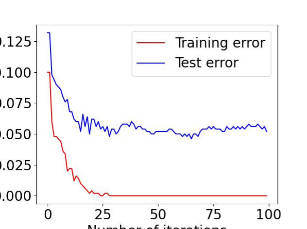
Results
Training Error dropped to 0 within ~30 iterations.
Test Error plateaued around 4–5%, indicating strong generalization performance.
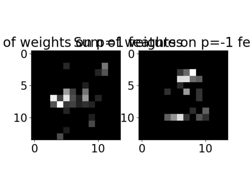
Visualization of the final classifier shows where the model focused its attention. Pixels along the middle and top diagonal regions were most influential for classifying “4”.
3 Programming: Kernel regression (a) Create a Python script gaussian vis.py for the following. Perform kernel regression using the Gaussian kernel: g(u) = 1 √ 2πh2 exp(−u2/(2h2)) n(:,3). Fit a regression model using h = {0.01,0.1,1,2,3,4}. Produce plots of the training data points, learned regression function, and test data points. The code visualize 1d.py in HW1 might be useful. Put 2 or 3 of these plots, for interesting (high values/low values of h) results, in your report. Include brief comments
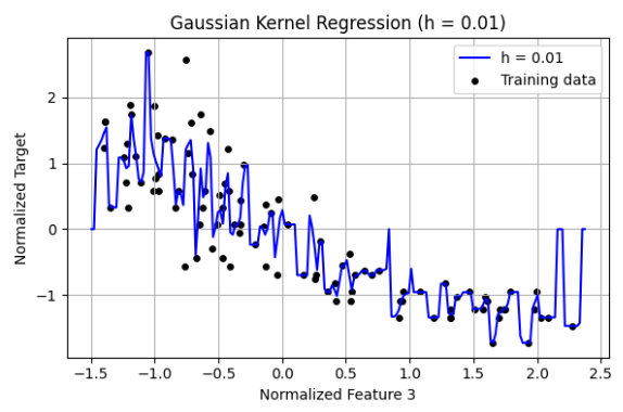
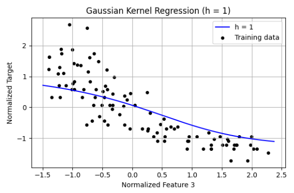
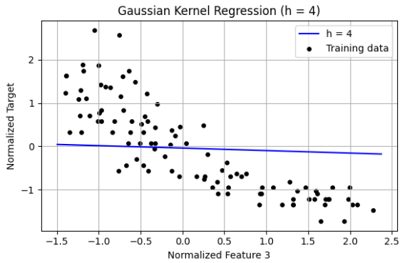
Observations Small Bandwidth h = 0.01 The regression curve is highly sensitive to individual training points. The curve is very wiggly and overfits the training data. h leads to low bias but high variance. The model fits noise and lacks generalization. Moderate Bandwidth h = 1 The regression line captures the general trend of the data. Smooth curve follows the underlying relationship well. This value of h provides a good bias-variance tradeoff. Large Bandwidth h = 4 The regression output is nearly a flat line. The model underfits and ignores meaningful variations in the data. h results in high bias and low variance, oversmoothing the data. The bandwidth h is a critical hyperparameter in kernel regression:
Too small → overfitting. Too large → underfitting. Just right → captures trend without modeling noise.h=1 is optimal for this feature and dataset.
(b) Create a Python script gaussian validate.py for the following. Again, perform the kernel regression using the Gaussian kernel with h = {0.01,0.1,0.25,1,2,3,4}. Use 10-fold cross-validation to decide on the best value for h. Produce a plot of validation set error versus h. Use a semilogx plot, putting h value on a log scale. Put this plot in your report, and note which h value you would choose from the cross-validation.
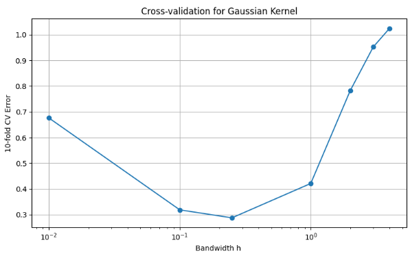
The figure shows the cross-validation error against h, using semilogx: Left side (h too small): Errors are high due to overfitting too sensitive to local noise. Middle (h ≈ 0.25): Lowest cross-validation error, indicating the best bias-variance tradeoff. Right side (h too large): Error increases due to underfitting too smooth to capture structure. Best Bandwidth h: 0.25, which gives the lowest 10-fold CV error.
(c) Create a Python script epanechnikov vis.py for the following. Repeat the experiment in (a), but this time use the Epanechnikov kernel: 3 g(u) = 4(1 −u2/h2) if |u|/h ≤ 1; 0 otherwise Include corresponding plots and brief comments in your report.
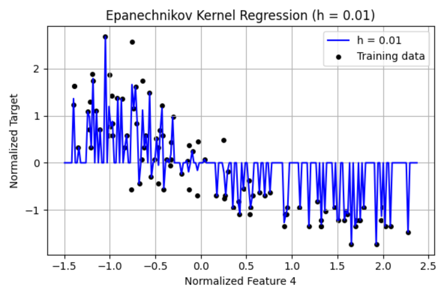
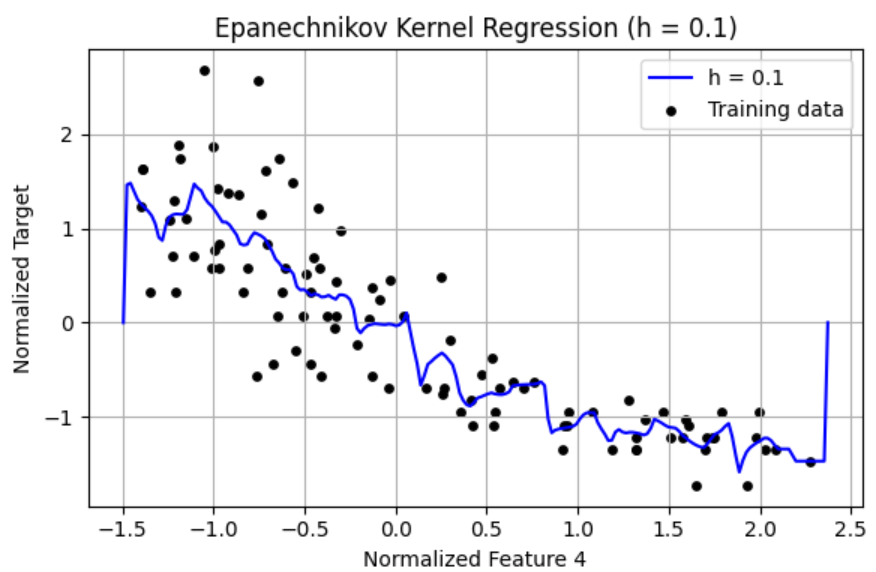
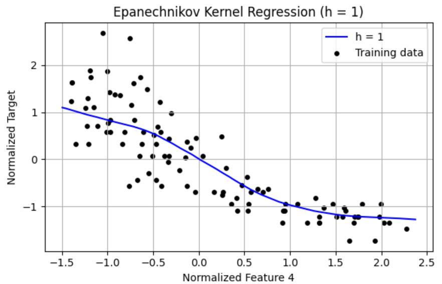
Results 1. h = 0.01 The curve fluctuates wildly and overfits the training data. Very high variance, memorizes noise. Severe overfitting, poor generalization. 2. h = 0.1 Smoother curve, but still shows sensitivity to local noise. Overfitting is reduced but still present. Slight improvement in generalization. 3. h = 1 Smooth, interpretable curve capturing the underlying trend. Excellent fit that avoids both over and underfitting. Best bias-variance tradeoff visually. Very small h 0.01 leads to overfitting. Large h 3–4 tends to oversmooth. h=1 produces the best result visually for the Epanechnikov kernel.
(d) Create a Python script epanechnikov validate.py for the following. Repeat the experiment in (b), but this time use the Epanechnikov kernel. Put the cor responding in your report, and note which h value you would choose from the cross-validation
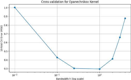
The plot shows the cross-validation error versus h using semilogx: Figure: Cross-validation Error vs Bandwidth h Very small h 0.01: High error due to overfitting. Very large ℎ h (3–4): Increasing error due to oversmoothing underfitting. Optimal range: h=0.25 and h=1 perform best. Minimum error occurs at h=1 . Conclusion The Epanechnikov kernel performs best with moderate bandwidths. The value h=1 minimizes the 10-fold CV error and achieves the best generalization.