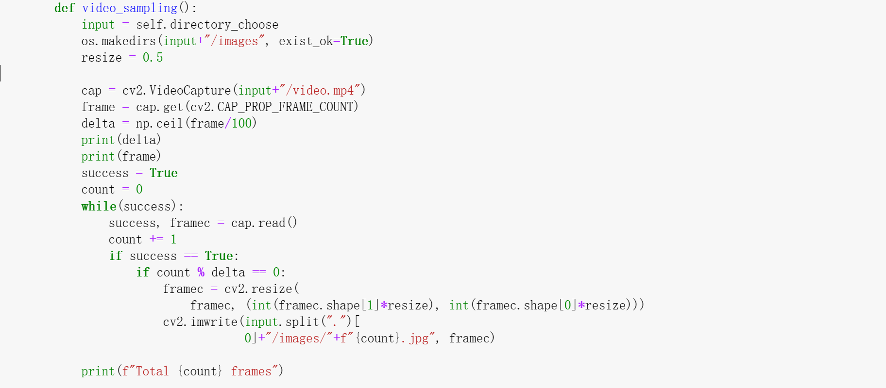
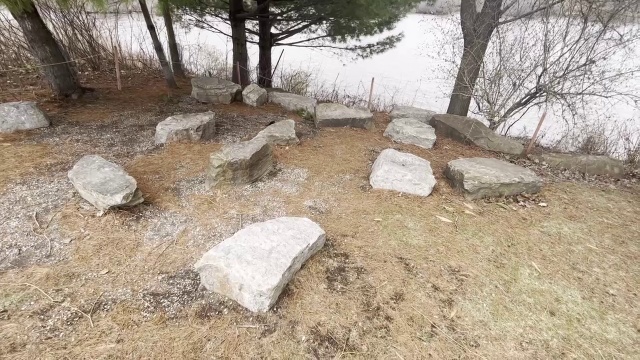
The Python function video_sampling() subsamples a video and extracts its frames as images.
It takes the "video.mp4" input video file from a specified directory and constructs
a "images" subdirectory to store the extracted frames. The function reads the video
using the OpenCV VideoCapture class and calculates the sampling interval (delta) based
on the overall number of frames. The programme then iterates through the video frames
and resizes the chosen ones by a predefined factor (in this case, 0.5). The resized
frames are then stored as separate image files within the "images" subdirectory. This
uncomplicated and effective implementation enables users to subsample a video and convert
it into a sequence of images for further processing or analysis.
The robust open-source computer vision toolkit known as OpenCV
can be utilised for the purpose of processing and modifying films
in an effective manner. OpenCV can be used to read the video frames
and save them at a reduced frame rate, which allows a video to have
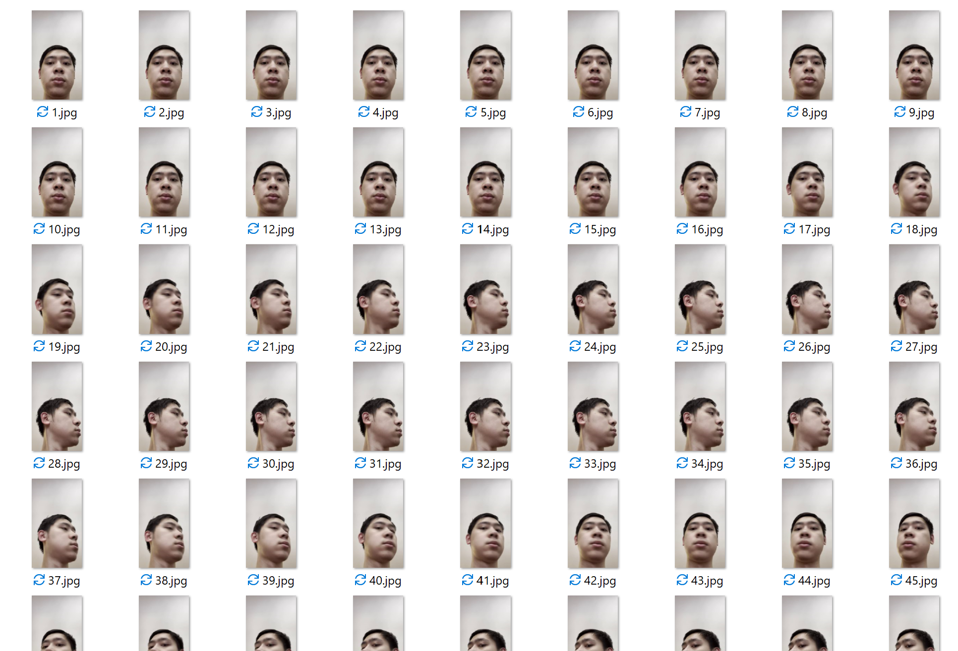
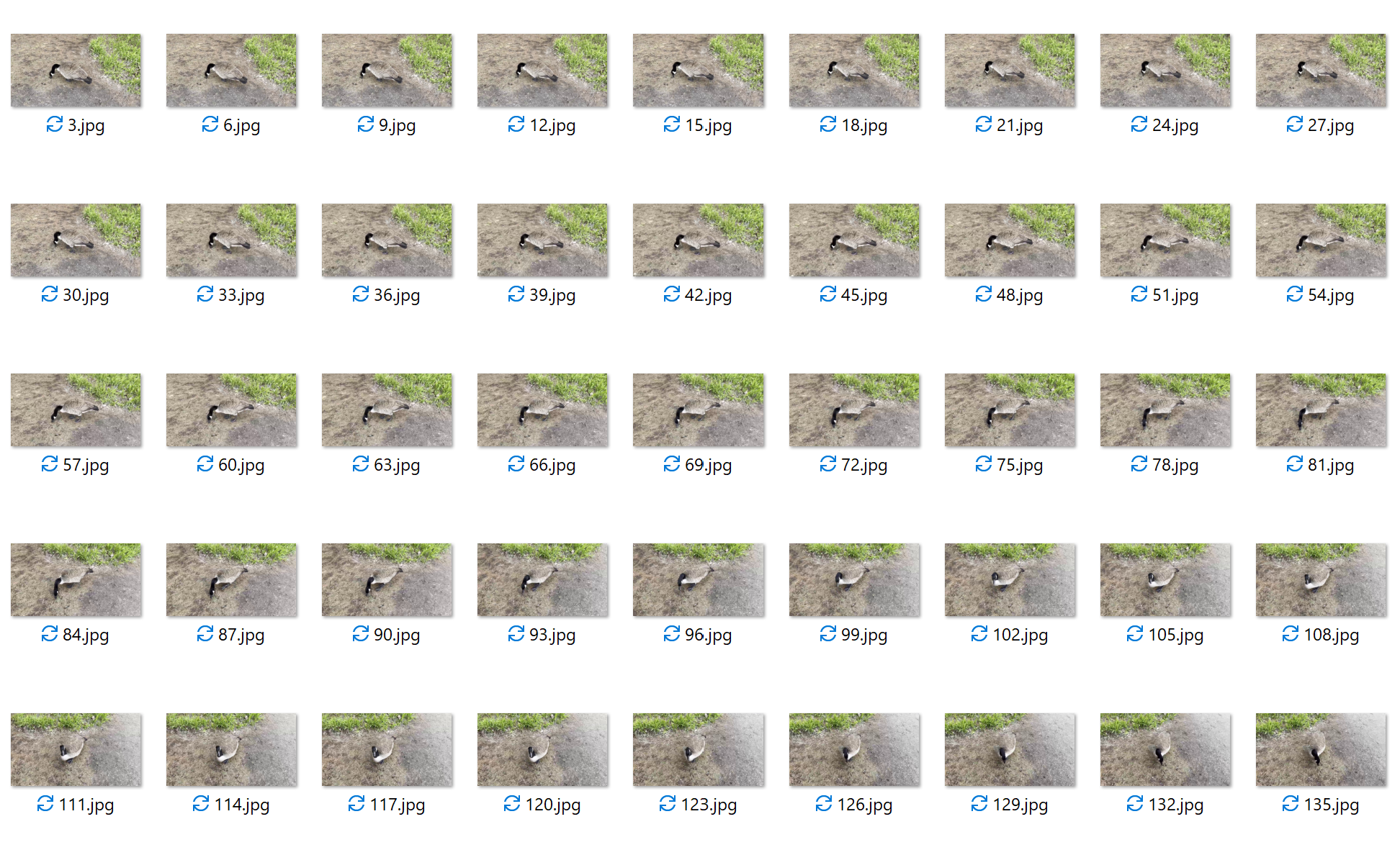
its frames subsampled and then be divided up into numerous images.
As each frame is iterated through, it is possible to extract the
images from it and save them as separate files in a directory of
your choosing. This method makes it possible to compile a set of still
images from the video, which can then be used for a variety of purposes,
such as frame-by-frame analysis, image processing, or the training of machine
learning models. The process of subsampling a video and converting it into a
sequence of images may be accomplished with relative ease with only a few lines
of code because to OpenCV's extensive collection of functions and user-friendly application programming interface .
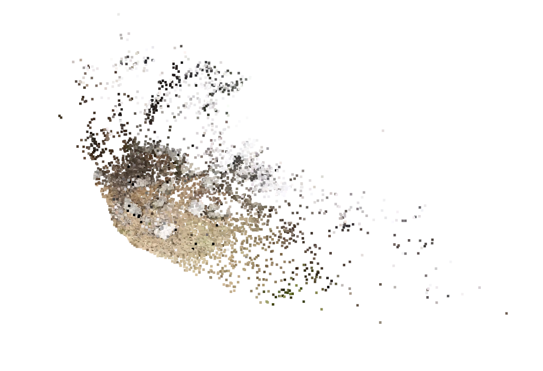
Sparse Reconstruction
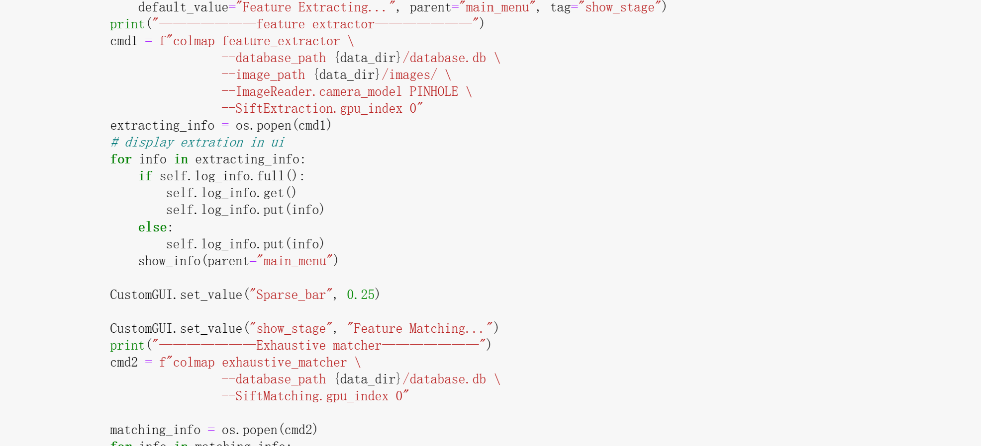
In my sparse reconstruction pipeline, three main steps are involved: feature extraction, exhaustive matching, and location mapping. Here's a detailed explanation of how each step works:
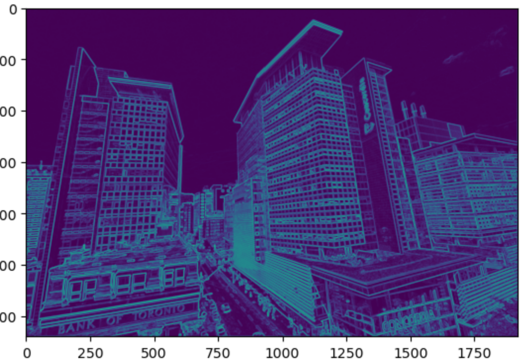
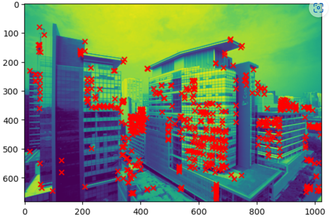
Feature extraction: This step is responsible for detecting distinct and repeatable keypoints (or features) in the input images,
which can be used for matching corresponding points across different images.
A feature descriptor is computed for each keypoint, capturing its local appearance information.
There are several popular feature extraction algorithms, such as SIFT, SURF, ORB, and AKAZE.
These algorithms are designed to be robust to changes in scale, rotation, and illumination.
In this assignment I use SIFT extraction.
Feature extraction is a critical step in the sparse reconstruction pipeline,
as it provides the basis for finding matches between images and establishing correspondences for triangulation and 3D point estimation.
sift gradiant
sift feature extract
Exhaustive matcher: The exhaustive matching step takes the feature descriptors from all input images
and compares them pairwise to find the best matches. By calculating the similarity between feature descriptors,
it determines which keypoints correspond to the same 3D point in the scene.
In the exhaustive approach, all possible image pairs are matched, which can be
computationally expensive for large image sets. However, it provides a high degree of certainty that the
correct matches are found, contributing to a more accurate and reliable reconstruction.
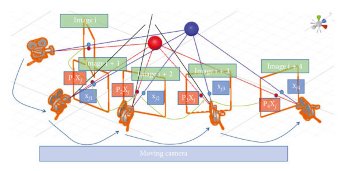
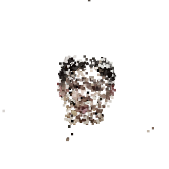
Location mapper: After obtaining the matched keypoints across images,
the location mapping step is responsible for estimating the 3D positions
of the keypoints and the camera poses (location and orientation) for each input image.
This is usually achieved using a combination of triangulation and bundle adjustment techniques.
Triangulation involves estimating the 3D coordinates of a point by intersecting the corresponding rays
from multiple camera viewpoints. Bundle adjustment is an optimization process that refines both the 3D
point locations and camera poses by minimizing the reprojection error, which is the difference between the observed
and projected 2D feature locations in the images. The location mapper outputs the 3D structure (sparse point cloud) and
camera poses, which together form the basis of the sparse reconstruction.
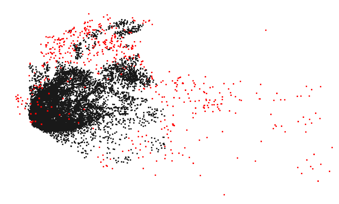
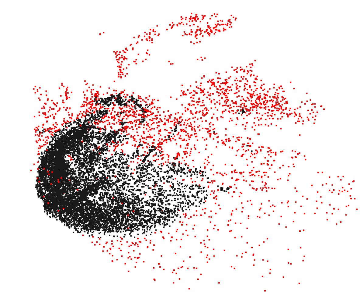
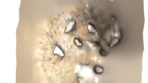
Point Cloud Operation-Outliers
you can use two popular outlier removal methods to clean up point cloud data: radius outlier removal and statistical outlier removal.
adius outlier removal: This method filters the point cloud based on the local point density within a specified radius. For each point in the point cloud, it counts the number of neighboring points that fall within the given radius. If the number of neighbors is less than a user-defined threshold, the point is considered an outlier and removed from the point cloud. Radius outlier removal effectively reduces noise and retains the main structure of the point cloud.
Statistical outlier removal: This method removes points that have a significantly different average distance to their neighbors compared to the overall point cloud. It calculates the mean and standard deviation of the distances from each point to its neighbors within a given search radius. Points with an average distance beyond a user-defined factor times the standard deviation are considered outliers and removed. Statistical outlier removal is more robust to varying point density and can effectively remove noise and outliers.
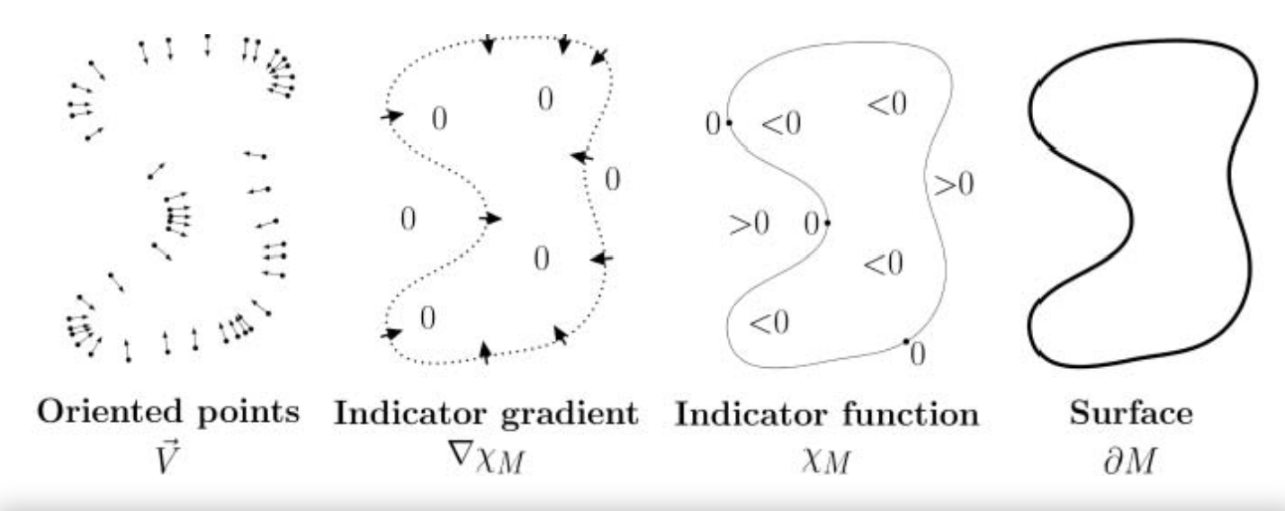
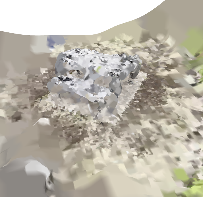
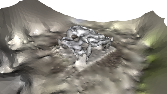
Poisson reconstruction
Input: The point cloud along with its associated
normals is what the Poisson reconstruction method receives as its input. Estimating these
normals is possible through the use of a variety of approaches, such as the principle component
analysis (PCA) or the least squares fitting of the local planes. Important directional information that helps guide the process of surface reconstruction is provided by the normals.
Estimation of the gradient field The procedure begins by doing an
estimation of the gradient field using the input point cloud and the normals.
Calculating the gradients of a scalar function that is meant to approximate the indicator function of the object is how this is accomplished. The indicator function returns a value of 0 while it is outside of the object but returns 1 when it is within. At the locations where the point cloud is located, the gradient of the scalar function should be relatively near to the provided normals.
Laplacian
The next step is to develop a Poisson equation that
relates the Laplacian of the scalar function (a measure of its curvature)
to the divergence of the estimated gradient field. This will be accomplished by
formulating a Poisson equation that relates the two quantities. An example of a partial differential equation is the Poisson equation. When this equation is solved, the result is a smooth scalar function that provides an approximation of the indicator function of the object.